Kalman Filter, extended version and no derivative required version

Before jumping into Kalman filter, we should recall Gaussian distribution and its effectiveness when digital computers not ready yet.

Gaussian pdf function for a random variable x ~ \(N\) ( \(m\), \(P\))

\[N( x | m, P) = \frac{1}{(2\pi)^{n/2} P^{1/2}} \exp{(-\frac{1}{2} (x - m)^T P^{-1} (x- m))}\]

Let x and y have the Gaussian densities and have linear relationship

\[P(x) = N(x | m, P )\] \[P(y|x)= N(y|Hx, R)\]

The joint and marginal distribution of x and y are given as follows:

\[\begin{pmatrix} x \\\ y \end{pmatrix} \sim N \left( \begin{pmatrix} m\\\ Hm\end{pmatrix}, \begin{pmatrix} P && PH^{T}\\\ HP && HPH^T + R\end{pmatrix}\right)\] \[y \sim N(Hm, HPH^T + R)\]

Suppose that you have a system with a bunch of variables with linear relationship. We can utilize the above equations to get the marginal distributions and conditional distributions of x and y as follows:

\[x|y \sim N(m + PH^T(HPH^T+R)^{-1}(y - Hm), P - PH^T(HPH^T + R)^{-1}HP)\]

You don’t need to memorize all above equations, just need to understand that with two random variables x and y are normally distributed and have linear relationship we can have all other marginal and conditional distributions followed Gaussian distributions respectively. That sounds great ?! Because if you lived in 18th and 19th century, you did NOT have computers or neural networks (or its variations called Deep NN) so at that time Gaussian distributions showing off its effectiveness in computing marginal or conditional distributions.

#Kalman Filter and its relation to Markov chain and Gaussian distributions But What is Kalman filter, why am I talking too much about Carl Friedrich Gauss. Ok, take a deep breath and see the procedure of combining Markov chain and Gaussian to solve the problem of estimating the state of a system using Kalman filter.

Let’s make a motivation example to understand better about these above fashion terms: you’ve built a legged robot that can wander in your home and the robot should knows where it is to avoid colliding with many obstacles.

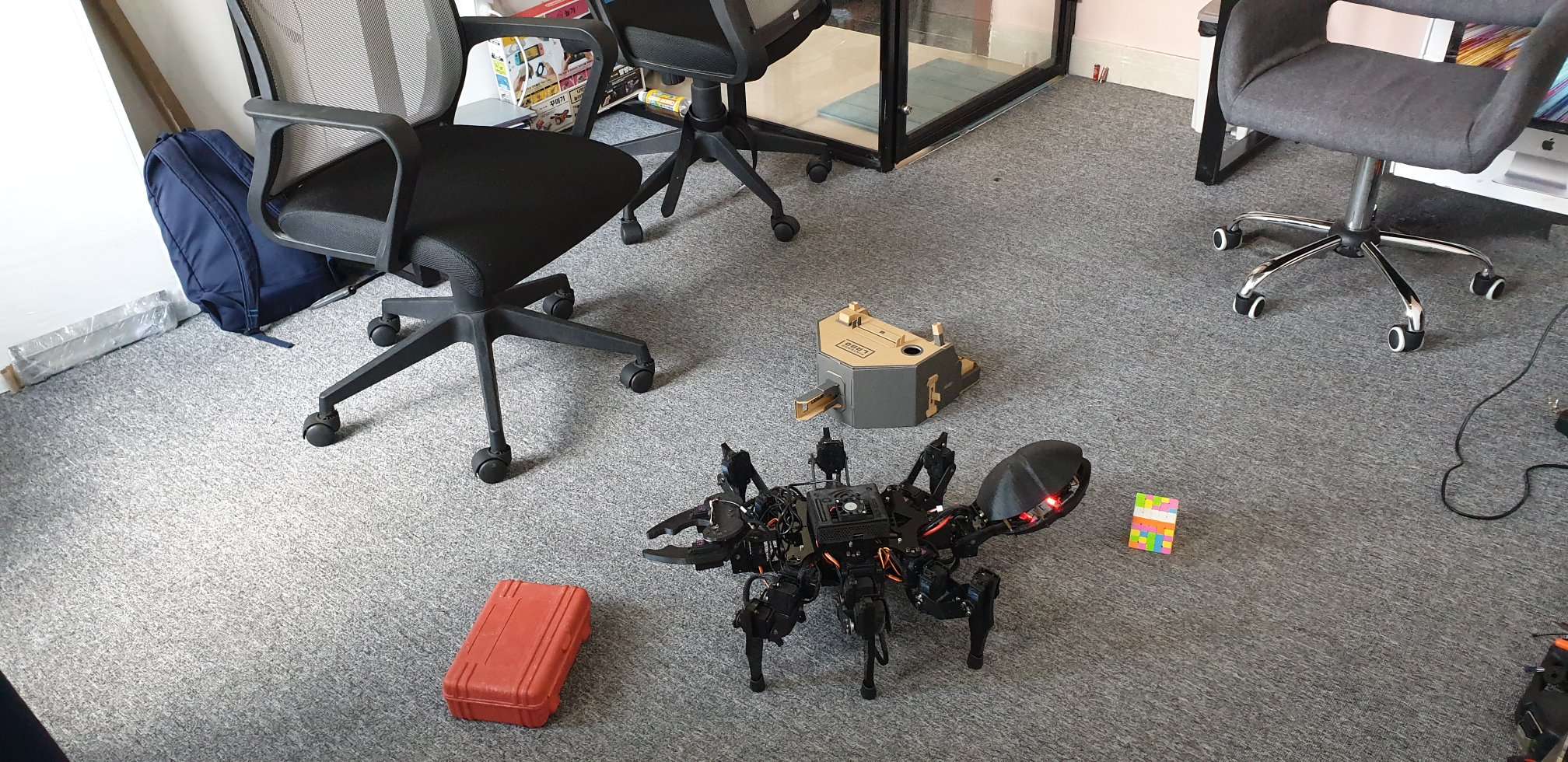
We can assume that the robot has state x consists of a position and a velocity. You can add more variables to the state vectors such as temperature of the engine, amount of battery in the power part of your robot or any variables that makes senses to track.

\[x = \begin{pmatrix} p \\\ v \end{pmatrix}\]

The robot also have a GPS sensor which is assumed to be accurate about 10 meters. As you know in your home there are a lot of obstacles and your robot can hit or be trapped in between those obstacles. 10 meters in accuracy is a huge number since your home may be 11 meters wide. So we need more information to determine the state x of our robot.

Because you are the programmer and hardware nerd to create the robot, you know about the commands sent to the wheel motors with a velocity and/or direction vectors. We know that the next time step the robot will likely to move. But of course we can not determine the environment surrounding the robot such as the bumpy terrain of your home or a new home, the obstacles may be moved by any members of your family, etc.

The main question is: How can the robot automatically navigate in the unpredicted environments? (autonomous agent ha)

Before mathematically speaking about the problem, let’s assume several conditions for the state of the robot and its measurement (GPS or any computer vision tracking object coordinates)

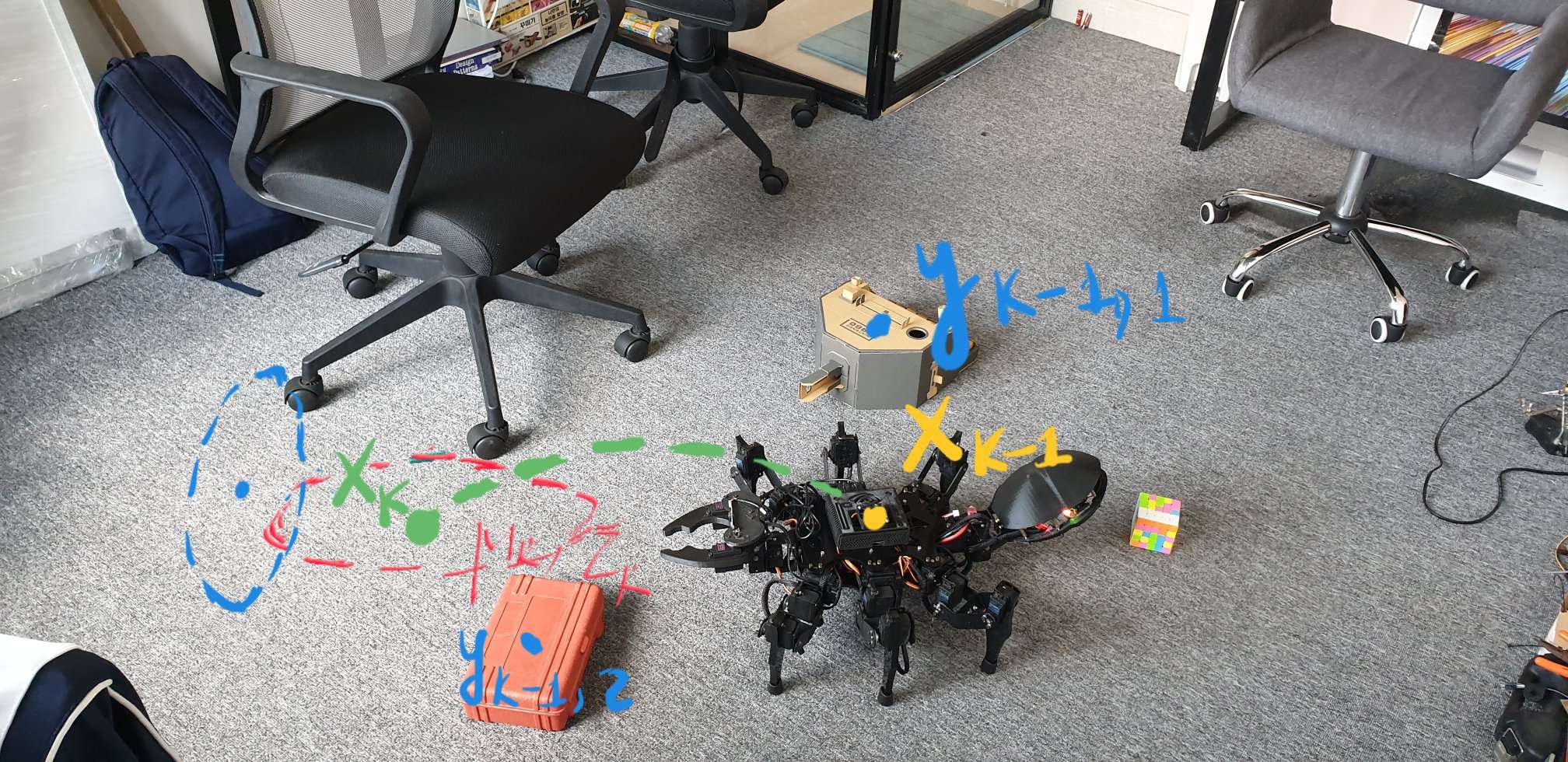
Formulate the problem The problem can be formulated as general probabilistic state space model:

• Measurement model: \(y_{k} \sim p(y_{k} \mid x_{k})\)

• Dynamic model: \(x_{k} \sim p(x_{k} \mid x_{k-1})\)

  The state space mode has the form of hidden Markov model (HMM): observed

Prediction step via Chapman-Kolmogorov equation

\[P(x_k | y_{1:k-1}) = \int p(x_k|x_{k-1}) p(x_{k-1} | y_{1:k-1}) dx_{k-1}\]

Update step

\[p(x_k | y_{1:k}) = \frac{1}{Z_k} p(y_{k}|x_k, y_{1:k-1}) p(x_k|y_{1:k-1})\]

Markovian assumption

\[p(x_k | y_{1:k}) = \frac{1}{Z_k} p(y_{k}|x_k) p(x_k|y_{1:k-1})\]

and \(Z_{k} = p(y_{k} \mid y_{1:k-1})\) is given as

\[Z_k = \int p(y_k |x_k)p(x_k|y_{1:k-1})dx_k\]

Let’s think about Kalman filter as a Bayesian filtering with Gaussian-Markov model.

\[x_k = A_{k-1}x_{k-1} + q_{k-1} = f(x_{k-1}, q_{k-1})\] \[y_k = H_k x_k + r_k = g(x_k, r_k)\]

• \(q_{k-1} \sim N(0, Q_{k-1})\) white process noise
• \(r_k \sim N(0, R_k)\) white measurement noise
• \(A_{k-1}\) is the transition matrix
• \(H_k\) is the measurement model matrix

We can express these above equations in probabilistic language as follows:

\[p(x_{k} \mid x_{k-1}) = N(x_{k} \mid A_{k-1} x_{k-1}, Q_{k-1})\] \[p(y_{k} \mid x_{k}) = N(y_{k} \mid H_{k} x_{k}, R_{k})\]

Derivation of the prediction step in Kalman filter Follows the Chapman-Kolmogorov equation, we can get

\[p(x_k|y_{1:k-1}) = \int p(x_k|x_{k-1}) p(x_{k-1 | y_{1:k-1}})dx_{k-1} = \int N(x_k|A_{k-1}x_{k-1}, Q_{k-1}) N(x_{k-1}|m_{k-1}, P_{k-1})\]

We all know that the answer for the above equation will be another Gaussian distribution

\[p(x_k|y_{1:k-1}) = N(x_k|A_{k-1}m_{k-1}, A_{k-1}P_{k-1}A_{k-1}^T + Q_{k-1}) = N(x_k|m_k^-, P_k^-)\]

Derivation of the update step in Kalman filter

the joint distribution of \(y_k\) and \(x_k\) is

\[p(x_k, y_k|y_{k-1}) = N(\begin{bmatrix} x_{k} \\ y_{k} \\ \end{bmatrix} | m^{''}, P^{''})\]

where

\[m^{''} = \begin{pmatrix} m_k^- \\\ H_k m_k^- \end{pmatrix}\] \[P^{''} = \begin{pmatrix} P_k^- && P_k^-H_k^T \\\ H_k P_k^- && H_k P_k^- H_k^T + R_k \end{pmatrix}\]

The conditional distribution \(p(x_{k} \mid y_{1:k})\) is given as

\[p(x_k|y_k, y_{1:k-1}) = N(x_k |m_k, P_k)\]

where

\[S_k = H_k P_k^- H_k^T + R_k\] \[K_k = P_k^- H_k^T S_k^{-1}\] \[m_k = m_k^- + K_k [y_k - H_k^- m_k^-]\] \[P_k = P_k^- - K_k S_k K_k^T\]

I already told you NOT to remember equations. Since we can derive it ourselves ha?!

What we need to care about is the weakness of the algorithm to know when it should be utilized to solve real problems.

• Kalman filter can be applied to the linear Gaussian models. Recall the state space model equations for more details.
• What if \(x_k\) and \(y_k\) are not Gaussian random variables ? It seems that the Gaussian assumption is too strict.