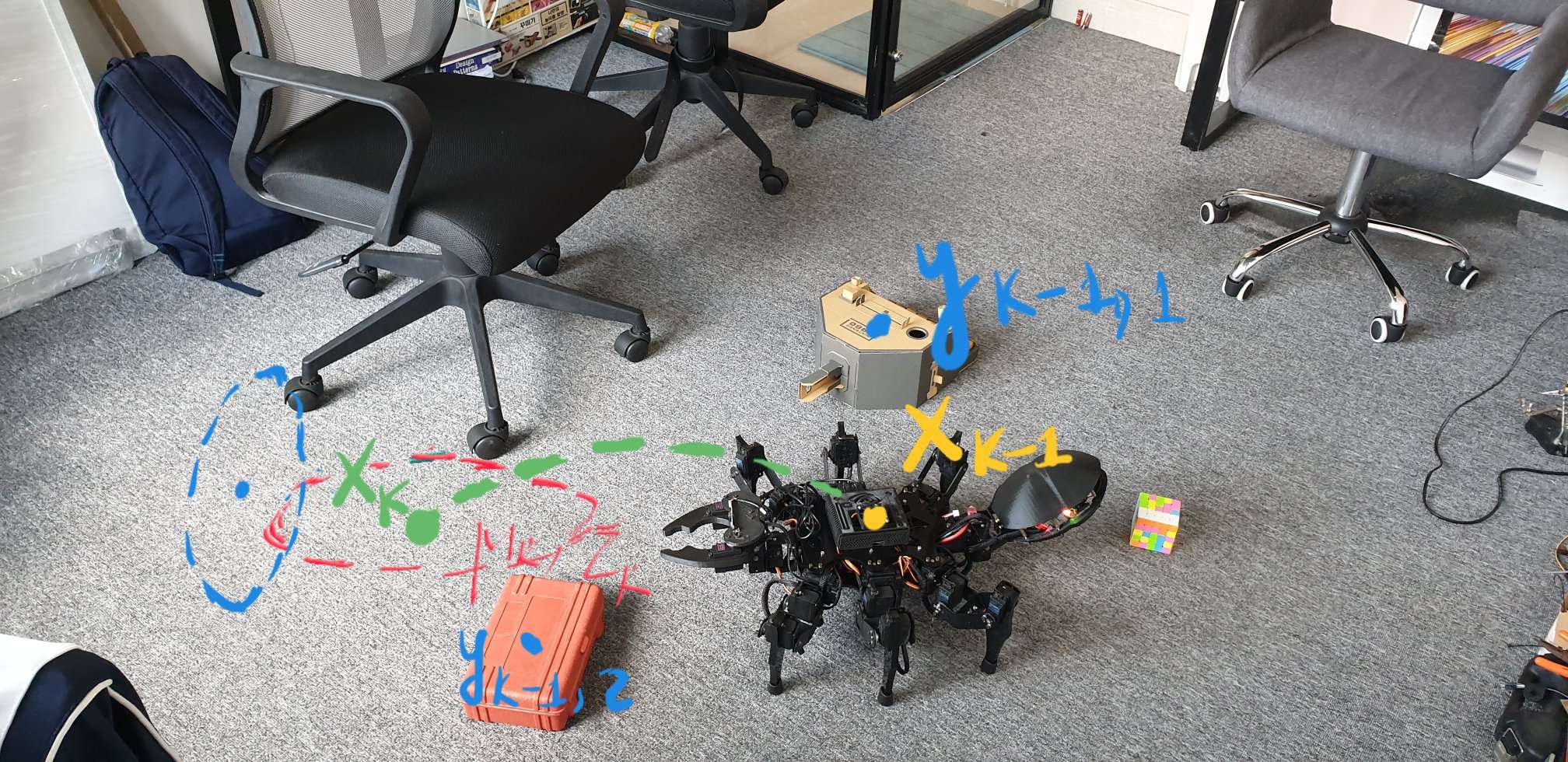
- \(f(.)\) is the dynamic model function or the prediction model
- \(h(.)\) is the observation model or the measurement model function
- \(r_k \sim N(0, R_k)\) is Gaussian measurement noise may be from your Computer Vision module
- \(q_{k-1} \sim N(0, Q_k)\) is Gaussian process noise may be from your control module
The non-linear functions can be linearized as follows:
\(f(x) \approx f(m) + F_x(m) (x-m)\) \(h(x) \approx h(m) + H_x(m) (x-m)\)
where \(x \sim N(m, P)\) and \(F_x, H_x\) are the Jacobian matrices of \(f\) and \(h\), respectively.
Let’s consider a base case - a transformation of \(x\) into \(y\)
\[x \sim N(m,P)\] \[y = g(x)\]We should ask the main questions of Linear Approximation of Non-Linear Transforms are what is the mean and covariance of \(y = g(x)\)
First, the probability density of y is now NOT Gaussian any more. The main reason is that the form of it is now as follows:
\[p(y) = \mid J(h)\mid N(g^{-1}(y) \mid m, P)\]But we should linearly approximate the probability distribution of \(y = g(x)\) by estimating its mean \(E[g(x)]\) and its covariance \(Cov[g(x)]\)
Utilizing Taylor series expansion of \(g\) on mean \(m\), we can get:
\[g(x) = g(m + \delta x) = g(m) + G_x(m) \delta x + \sigma_i \frac{1}{2}\delta x^T G_{xx}^(i)(m)\delta x\]where \(\delta x = x-m\)
Linear approximation:
\[g(x) \approx g(m) + G_x(m)\delta x\] \[E[g(x)] \approx g(m) + G_x(m) E[ \delta x] \approx g(m)\]For covariance we get the approximation based on Delta method for multivariate variables
\[g(x) \approx g(m) + G_x(m)^T (x-m)\] \[\begin{eqnarray} Var[g(x)] &\approx& Var[g(m) + G_x(m)^T (x-m)] \\\\\\ &=& Var[g(m) + G_x(m)^T x - G_x(m)^T m] \\\\\\ &=& Var[G_x(m)^T x] \\\\\\ &=& G_x(m)^T Var(x) G_x(m) \end{eqnarray}\] \[cov[g(x)] \approx G_x(m)^T P G_x(m)\]Now, we derive the EKF based on the linear approximations of non-linear transforms.
#Prediction step
Assume that the filtering distribution of the previous step is Gaussian
\[p(x_{k-1} \mid y_{1:k-1}) \approx N(x_{k-1} \mid m_{k-1}, P_{k-1})\]The joint distribution of \(x_{k-1}\) and \(x_k = f(x_{k-1}) + q_{k-1}\) is NOT Gaussian anymore since \(f()\) is non linear function. We can approximate linearly as follows:
\[p(x_{k-1}, x_k \mid y_{1:k-1}) \approx N( \left [ x_{k-1}, x_k \right ] \mid m^{'}, P^{'})\]where
\[m^{'} = \begin{pmatrix} m_{k-1} \\\ f(m_{k-1}) \end{pmatrix}\] \[P^{'} = \begin{pmatrix} P_{k-1} && P_{k-1}F_x^T(m_{k-1}) \\\ F_x(m_{k-1})P_{k-1} && F_xP_{k-1}F_x^T + Q_{k-1} \end{pmatrix}\]In the prediction step, the approximate predicted distribution of \(x_k\) given \(y_{1:k-1}\) is Gaussian with moments
\[P(x_k \mid y_{1:k-1}) \sim N(m_k^{-}, P_{k}^{-})\] \[m_k^{-} = f(m_{k-1})\] \[P_k^{-} = F_xP_{k-1}F_x^T + Q_{k-1}\]#Update step Similarly, we can approximate the joint distribution of \(x_k\) and \(y_k = h(x_k) + r_k\) by linear approximation although the distribution is non-Gaussian
\[P(x_k, y_k \mid y_{1:k-1}) \approx N \left( \begin{matrix} x_k \\\ y_k \end{matrix} \mid m^{''}, P^{''} \right)\]where
\[m^{''} = \begin{pmatrix} m_k^{-} \\\ h(m_k^{-}) \end{pmatrix}\] \[P^{''} = \begin{pmatrix} P_k^{-} && P_k^{-}H_x^T(m_k^{-}) \\\ H_x(m_k^{-}) P_k^{-} && H_x(m_k^{-}) P_k^{-}H_x^T(m_k^{-}) + R_k \end{pmatrix}\]From the joint distribution, we can derive the conditional distribution \(p(x_k \mid y_k, y_{1:k-1}) \approx N(m_k, P_k)\) as follows:
\[m_k = m_k^{-} + P_k^{-} H_k^T (H_x P_k^{-} H_x^T +R_k)^{-1} [y_k - h(m_k^{-})]\] \[P_k = P_k^{-} - P_k^{-}H_x^T(H_x P_k^{-} H_x^{T} + R_k)^{-1}H_x P_k^{-}\]It sounds mathematically complex right?! But you don’t have to remember the equation since computers or edge computing resources will do it for you.
What we should understand and remember are the advantages and limitations of EKF.
- Noise processes must be Gaussian - not sure in real practices
- Jacobian matrices can be computationally expensive and quite error prone