Variational Methods and Image Segmentation (Part 1)

Snakes: Active Contours Models

Convolution neural networks usually appear in segmentation problems because of its high adaptation to many datasets and high performance. However, in return, they require ground truth data to learn and perform specific tasks, without ground truth their results are really poor. Today, we will introduce to you an “old” segmentation method but it can be applied in several certain problems in absence of datasets. This is called Snakes: Active Contours Models.

Formulation

Let \(I: \Omega \rightarrow \mathbb{R}\) be a gray scale image, where \(\Omega \subset \mathbb{R}^2\). The curve that segments image $I$ into 2 partitions is denoted as \(C: [0, 1] \rightarrow \Omega\), in other words \(C = (x(s), y(s))\) where \(s \in [0, 1]\).

There are innumerable curves \(C\), so how do we know which one is the most suitable for a given image? To answer that, Kass et al [1] proposed an energy function \(E(C)\) and the process of finding \(C\) is minimizing \(E(C)\):

\[E(C) = E_{int}(C) + E_{image}(C)\]

The internal energy \(E_{int}(C)\) contains 2 small terms:

• Continuity term: \(E_{cont}(C) = \int_0^1 |C_s|^2 \, ds = \int_0^1 \left|\dfrac{\partial x}{\partial s}\right|^2 + \left|\dfrac{\partial y}{\partial s}\right|^2 ds\)

• Smoothness term: \(E_{curve}(C) = \int_0^1 |C_{ss}|^2 \, ds = \int_0^1 \left|\dfrac{\partial^2 x}{\partial s^2}\right|^2 + \left|\dfrac{\partial^2 y}{\partial s^2}\right|^2 ds\)

The purpose of the energy is penalizing the non - continuos and non - smooth curve:

\[E_{int}(C) = \int_0^1 \alpha(s) |C_s|^2 + \beta(s) |C_{ss}|^2 \, ds\]

The external energy forces the curve toward to the boundary of the given image.

\[E_{img}(C)= -\int_0^1 |\nabla I(C)|^2 \, ds = - \int_0^1 I_x^2 + I_y^2 \, ds\]

If the curve is at the flat background, the magnitude of image gradient is zero, while when the curve is at boundary, the magnitude is the largest. Because of this, the external energy is negative of image gradient magnitude.

The total energy function needed to minimize is:

\[E(C) = \dfrac{1}{2} \int_0^1 - |\nabla I(C)|^2 + \alpha (s) |C_s|^2 + \beta (s) |C_{ss}| \, ds\]

Solution

Euler - Lagrange equation

What we need to find right now is not finite number of parameters but actually the function \(C\) and how we minimize energy function \(E\) where \(C\) is an argument?

According to Euler - Lagrange equation, the optimal function \(f\) must hold the necessary condition (Read more at here). The energy function can be written in the form:

\[\begin{equation} E(C) = \int_0^1L(C, C_s, C_{ss}) \, ds \end{equation}\]

And the necessary condition is:

\[\begin{equation} \dfrac{dE}{dC} = \dfrac{\partial L}{\partial Cs} - \dfrac{\partial}{\partial s}\left(\dfrac{\partial L}{\partial C_s}\right) + \dfrac{\partial ^ 2}{\partial s^2}\left(\dfrac{\partial L}{\partial C_{ss}}\right) = 0 \end{equation}\]

In fact, this necessary condition does not guarantee that the solution is global optimum but only local optimum. However, at least we still can find an acceptable solution by using gradient descent.

Continue to expand the above equation and get:

Since \(C = (x(s), y(s))\), we will take derivative two times, respect to \(x\) and to \(y\).

• \(x = x(s)\) \(\begin{aligned} \dfrac{dE}{dx} &= \dfrac{\partial L}{\partial x} - \dfrac{\partial}{\partial s}\left(\dfrac{\partial L}{\partial x_s}\right) + \dfrac{\partial ^2}{\partial s^2}\left(\dfrac{\partial L}{\partial x_{ss}}\right) \\ &= -(I_{x}I_{xx} + I_yI_{yx}) - \alpha (s) \dfrac{\partial x'}{\partial s} + \beta (s) \dfrac{\partial x''}{\partial s^2} \\ &= -(I_{x}I_{xx} + I_yI_{yx}) - \alpha (s) x^{(2)} + \beta (s) x^{(4)} \end{aligned}\)

where \(x^{(2)}\) and \(x^{(4)}\) respectively, are the second and fourth order derivative of \(x\) respect to \(s\).

• \(y = y(s)\) \(\begin{aligned} \dfrac{dE}{dy} &= \dfrac{\partial L}{\partial y} - \dfrac{\partial}{\partial s}\left(\dfrac{\partial L}{\partial y_s}\right) + \dfrac{\partial ^2}{\partial s^2}\left(\dfrac{\partial L}{\partial y_{ss}}\right) \\ &= -(I_{x}I_{xy} + I_yI_{yy}) - \alpha (s) y^{(2)} + \beta (s) y^{(4)} \end{aligned}\)

For the sake of simplicity, both weight parameters \(\alpha(s)\) and \(\beta(s)\) are considered as constant \(\alpha\) and \(\beta\).

Note: If you see some below expressions are a little bit challenging, you can read this blog this to have sense of how this method works.

Finite Difference

In reality, we define the curve \(C\) by a set of points \(\{x_i, y_i\}\) not by parametric functions, so to find \(x^{(2)}\) and \(x^{(4)}\), the central difference will be used. (Read more at here)

\[\begin{aligned} x^{(2)}(s) &\approx \dfrac{x(s + h) - 2x(s) + x(s-h)}{h^2} \\ x^{(4)}(s) &\approx \dfrac{x(s + 2h) - 4x(s + h) + 6x(s) - 4x(s-h) + x(s - 2h)}{h^4} \\ \end{aligned}\]

We can also rewrite these equations above in the matrix form.

\[\begin{equation} X^{(2)} \approx \left[\begin{array}{c} -2 & 1 & 0 & \cdots & 0 & 1 \\ 1 & -2 & 1 & \cdots & 0 & 0 \\ 0 & 1 & -2 & \cdots & 0 & 0 \\ \vdots & \vdots & \vdots & \ddots & \vdots & \vdots \\ 0 & 0 & 0 & \cdots & -2 & 1 \\ 1 & 0 & 0 & \cdots & 1 & -2\\ \end{array}\right] \left[\begin{array}{c} x_1 \\ x_2 \\ x_3 \\ \vdots \\ x_{n-1} \\ x_n \end{array}\right] = A_2 X \end{equation}\] \[\begin{equation} X^{(4)} \approx \left[\begin{array}{c} 6 & -4 & 1 & \cdots & 1 & -4 \\ -4 & 6 & -4 & \cdots & 0 & 1 \\ 1 & -4 & 6 & \cdots & 0 & 0 \\ \vdots & \vdots & \vdots & \ddots & \vdots & \vdots \\ 1 & 0 & 0 & \cdots & 6 & -4 \\ -4 & 1 & 0 & \cdots & -4 & 6\\ \end{array}\right] \left[\begin{array}{c} x_1 \\ x_2 \\ x_3 \\ \vdots \\ x_{n-1} \\ x_n \end{array}\right] = A_4 X \end{equation}\]

Finally, the term \(-\alpha x^{(2)} + \beta x^{(4)}\) in Euler - Lagrange equation above is rewriten as matrix form: \(-\alpha A_2 X + \beta A_4X\).

This is applied the same to \(Y^{(2)}\) and \(Y^{(4)}\).

Implicit Euler method

To simplify notation, let \(A = -\alpha A_2 + \beta A_4\) and \(P_x = I_xI_{xx} + I_yI_{yx}\).

The Euler - Lagrange equation becomes:

\[\dfrac{dE}{dX} = -P_x(X) + AX\]

In this step, we will use implicit Euler method and consider \(P_x(X)\) as constant:

\[\dfrac{1}{\gamma}(X_t - X_{t+1}) = -P_x(X_t) + AX_{t+1}\]

where \(\gamma\) is step size.

Finally, the \(X_{t+1}\) is obtained by:

\[X_{t+1} = (\gamma A + I_d)^{-1}(\gamma P_x(X_t) + X_t)\]

The update equation for \(Y_{t+1}\) is the same:

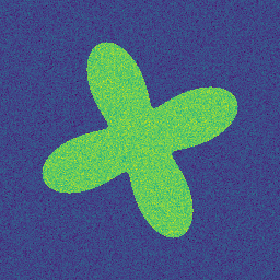
\[Y_{t+1} = (\gamma A + I_d)^{-1}(\gamma P_y(Y_t) + Y_t)\]

Results

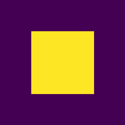
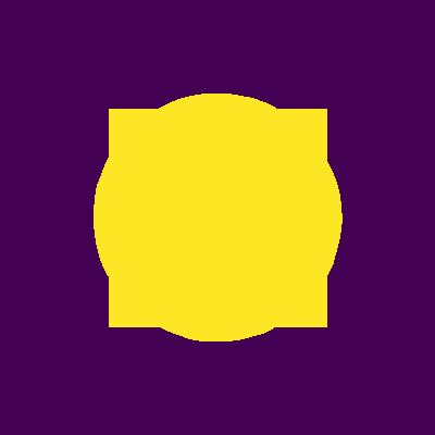
Input Images	Results

References

[1] Kass, Michael, Andrew Witkin, and Demetri Terzopoulos. “Snakes: Active contour models.” International journal of computer vision 1.4 (1988): 321-331.