Active Contours Without Edges
After finishing Snakes problem, we now get into an improvement of it which is called Active Contours Without Edges. The reason it has “without edges” is that the model doesn’t use the image gradient information of input image. You can also read the original version at here. We recommend you read other blogs in here, and here to understand the general idea and method used this solving branch.
Formulation
Let \(I: \Omega \rightarrow \mathbb{R}\) be a gray scale image, where \(\Omega \subset \mathbb{R}^2\). The curve \(C\) segments image \(I\) into 2 partitions: \(R_i\) the region inside \(C\), and \(R_o\) the region outside \(C\). Let us define the energy function evaluating the performance of segmentation:
\[E(C) = E_i(C) + E_o(C) = \iint_{R_i} |I(x,y) - c_i|^2 \, dx \, dy + \iint_{R_o} |I(x,y) - c_o|^2 \, dx \, dy\]where \(c_i\) and \(c_o\) respectively are the average \(I(x,y)\) in \(R_i\) and \(R_o\).
Intuitively, we can notice this energy function makes sense since:
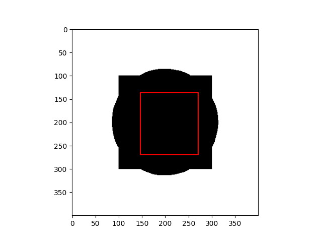
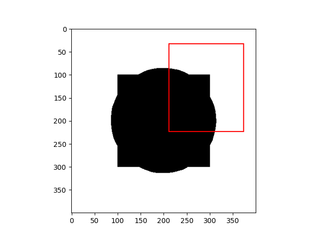
- If the curve \(C\) is inside an object, \(E_i \approx 0\) and \(E_o \gt 0\).
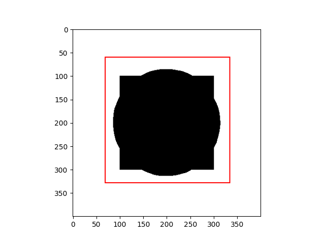
- If the curve \(C\) is outside an object, \(E_i \gt 0\) and \(E_o \approx 0\).
- If the curve \(C\) is both inside and outside an object, \(E_i \gt 0\) and \(E_o \gt 0\).
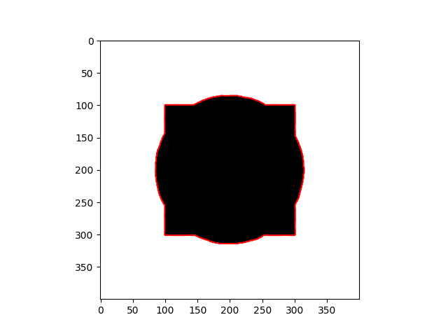
- If the curve \(C\) can segment an object perfectly, \(E_i \approx 0\) and \(E_o \approx 0\).
| Curve inside an object | Curve outside an object |
|---|---|
 |
 |
| Curve inside and outside an object | Curve fitting an object |
 |
 |
Similar to Snakes: Active Contours Model, TF Chan [1] would add some regularization terms into the energy function such as Length of curve \(C\) and (or) Area of \(R_i\). The final energy function will be:
\[\begin{aligned} E(C, c_1, c_2) &= \mu \, Length(C) + \nu \, Area(inside(C)) \\ &+ \lambda_1 \iint_{R_i} |I(x,y) - c_i|^2 \, dx \, dy \\ &+ \lambda_2 \iint_{R_o} |I(x,y) - c_o|^2 \, dx \, dy \end{aligned}\]The curcial step of this method is to replace an unknown curve \(C: [0, 1] \rightarrow \Omega \subset \mathbb{R}^2\) by an unknown surface \(\phi: \Omega \subset \mathbb{R}^2 \rightarrow \mathbb{R}\). The curve \(C\), region inside \(C\) \(R_i\) and outside \(C\) \(R_o\) can be re - defined:
\[\begin{equation*} \begin{cases} C &= \{(x, y) \in \Omega \, | \, \phi(x, y) = 0\} \\ inside (C) &= \{(x, y) \in \Omega \, | \, \phi(x, y) \gt 0\} \\ outside (C) &= \{(x, y) \in \Omega \, | \, \phi(x, y) \lt 0\} \end{cases} \end{equation*}\]We can compute length of curve \(C\) and area of region inside \(C\) by using heaviside step function and its derivative dirac delta function:
\[\begin{aligned} length(C) &= \iint_\Omega |\nabla H (\phi(x, y))| \, dx \,dy = \iint_\Omega \delta(\phi(x ,y))|\nabla \phi(x, y)| \, dx \,dy \\ Area(R_i) &= \iint_\Omega H(\phi(x, y)) \, dx \, dy \end{aligned}\]where:
- Heaviside step function is defined: \(\begin{equation*} H(x) = \begin{cases} 1 & \quad x \ge 0, \\ 0 & \quad x \lt 0. \end{cases} \end{equation*}\)
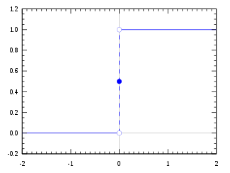
Heaviside step function
- Dirac delta function is dedined: \(\begin{equation*} \delta(x) = \begin{cases} \infty & \quad x = 0 \\ 0 & \quad \text{otherwise} \end{cases} \end{equation*}\)
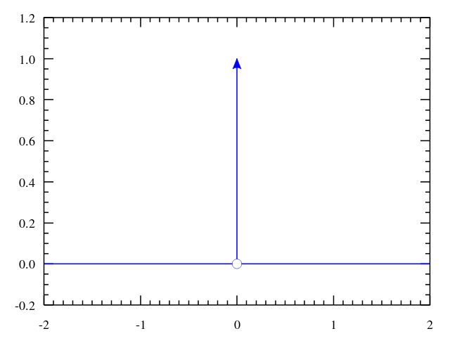
Dirac delta function
Finally, the energy function will be:
\[\begin{aligned} E(\phi, c_1, c_2) &= \iint_\Omega \mu \, \delta(\phi (x, y)) |\nabla \phi (x, y)| + \nu \, H(\phi (x, y))\\ &+ \lambda_1 H(\phi (x, y)) |I(x,y) - c_i|^2 + \lambda_2 (1 - H(\phi (x, y))) |I(x ,y) - c_o|^2 \, dx \, dy \end{aligned}\]Solution
Again, the method solving this problem is Euler - Lagrange Equation and gradient decent. We recommend you read the previous blog to familiarize yourself with the way we expand formulation.
\[\begin{aligned} E(\phi, c_1, c_2) &= \iint_\Omega \mu \, \delta(\phi (x, y)) |\nabla \phi (x, y)| + \nu \, H(\phi (x, y))\\ &+ \lambda_1 H(\phi (x, y)) |I(x,y) - c_i|^2 + \lambda_2 (1 - H(\phi (x, y))) |I(x ,y) - c_o|^2 \, dx \, dy \\ &= \iint_\Omega L(\phi, \nabla \phi, c_i, c_o) \, dx \, dy \end{aligned}\]The optimal \(\phi\), \(c_i\) and \(c_o\) are:
\[\begin{aligned} \underset{\phi, c_1, c_2}{\operatorname{arg\,min}} \, E(\phi, c_1, c_2) = \iint_\Omega L(\phi, \nabla \phi, c_i, c_o) \, dx \, dy \end{aligned}\]To solve this, first we would iteratively find optimal values/ function of each \(c_i\), \(c_o\) and \(\phi\):
- Step 1: Considering \(\phi\) and \(c_o\) as constants, the optimal value of \(c_i\) is: \(c_i = \dfrac{\iint_\Omega H(\phi (x, y)) I(x, y) \, dx \, dy}{\iint_\Omega I(x, y) \, dx \, dy}\)
-
Step 2: Considering \(\phi\) and \(c_i\) as constants, the optimal value of \(c_o\) is: \(c_o = \dfrac{\iint_\Omega (1 - H(\phi (x, y))) I(x, y) \, dx \, dy}{\iint_\Omega I(x, y) \, dx \, dy}\)
- Step 3: Considering \(c_i\) and \(c_o\) as constants, update step of \(\phi\) is: \(\dfrac{\partial \phi}{\partial t} = - \dfrac{dE}{d\phi} = \delta(\phi) \left( \mu \operatorname{div} \left(\dfrac{\nabla \phi}{|\nabla \phi|} \right) - \nu - \lambda_1 (I - c_i)^2 + \lambda_2 (I - c_o)^2 \right)\)
In implementation, rather having heaviside step and dirac delta function as discrete functions, we replace them by their softer versions:
\[\begin{aligned} H(x) &= \dfrac{1}{2}\left( 1 + \dfrac{2}{\pi} \operatorname{arctan}\left( \dfrac{x}{\epsilon}\right)\right) \\ \delta(x) &= \dfrac{\epsilon^2}{\pi(\epsilon^2 + x^2)} \end{aligned}\]where \(\epsilon = 10^{-6}.\)
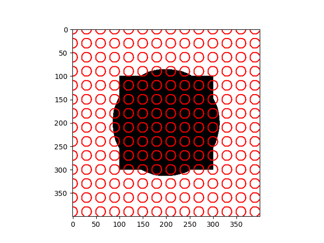
Results
| Input Images | Results |
|---|---|
 |
 |
 |
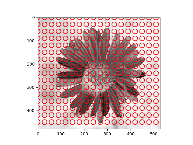 |
Discuss
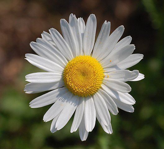
The method depends heavily on the initial \(\phi\) and the Euler - Lagrange equation is just a necessary condition which means it doesn’t guarantee that the optimum is global and sometimes the result is local optimum. As you can notice in the daisy flower sample, some regions in the background are recognized as foreground and the yellow disk flowers are the background.
Reference
[1] CHAN, Tony F.; VESE, Luminita A. Active contours without edges. IEEE Transactions on image processing, 2001, 10.2: 266-277.